GPU Accelerated Matrix Factorization for Recommender Systems

By: Doruk Kilitcioglu and Nick Greenquist

Introduction

Matrix Factorization (MF) is a popular algorithm used to power many recommender systems. Efficient and scalable MF algorithms are essential in order to train on the massive datasets that large scale recommender systems utilize. This blog post presents cu2rec, a matrix factorization algorithm written in CUDA. With a single NVIDIA GPU, cu2rec can be 10x times faster than state of the art sequential algorithms while reaching similar error metrics.

The code and the instructions on how to run it can be found on the GitHub page.

How It Works

In this section of this post, we will explain how what GPUs are, how they work, and how they can be used to accelerate a powerful algorithm commonly used for recommender systems: matrix factorization.

How do GPUs Work

Today, GPUs are being used more to more to parallelize algorithms that need to run on big data. GPUs have much more compute power than CPUs and work well performing the same instruction on multiple pieces of data (SIMD)¹. GPUs originally were used for heavy graphical work but have become a staple of large machine learning models². Because of the explosion of GPU usage across much of machine learning, we wanted to see if they could be useful in the sub-field of recommender systems.

GPUs are most useful when the task is computationally intensive, there are many independent computations, and the computations are similar. The architectural paradigm that most benefits from this is Single Instruction Multiple Data (SIMD), where a single instruction is executed for multiple data points.

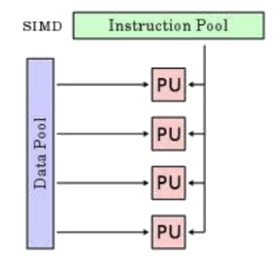
GPUs implement this SIMD architecture, but they do not devote the whole GPU to that instruction. Rather, only 32 execution units (out of 5000 in recent GPUs) have to execute the same instruction. The best practice is to structure your code to be as much SIMD as possible.

CUDA

CUDA is the programming language built by NVIDIA as a general purpose way of interacting with NVIDIA GPUs. It can be used with both C and C++, and gives the user API calls to important GPU functions such as copying data from and to GPU memory, and launching GPU functions called kernels.

Each kernel defines a function that is called per execution unit, called a thread. These threads are bundled into 32 units, called a warp. Each thread in a kernel executes the same function, but only these warps need to be simultaneously executing the same instruction. Furthermore, not all threads need to run concurrently, but they all need to finish before a kernel is done.

For more information about CUDA, you can check Kirk et al.¹.

Matrix Factorization for Recommender Systems

Matrix Factorization decomposes a rating matrix $R$ of shape $m\times n$ into two feature matrices, $P$ and $Q$. $P$ ($m\times f$) and $Q$ ($n\times f$), where $f$ is the number of factors, are the learned feature matrices. The goal of MF is to train the best $P$ and $Q$ matrices such that $R=P\times Q$, as shown in the figure below. In state of the art models, it also involves learning $U$ ($m\times 1$ matrix of user biases) and $I$ ($n\times 1$ matrix of item biases), with an additional global bias $\mu$ which is set to the mean of all ratings.

MF is incredibly popular and has been used for serving recommendations by companies such as Amazon and Netflix³. In the era of big data, the datasets that MF is being asked to tackle are getting orders of magnitude larger than even the Netflix Dataset⁴. In order to keep up, MF algorithms need to be fast, scalable, and able to handle massive amounts of data.

For more information, please look at these blog posts for a technical explanation of Matrix Factorization and an application of Matrix Factorization for book recommendation.

SGD for Matrix Factorization

For the task of rating prediction, we use the biased SVD popularized by Koren et al.⁵. For each user $u$ and item $i$ pair, the estimated rating $\hat r_{ui}$ and the error for that rating $e_{ui}$ are defined by:

\[\begin{eqnarray} \hat{r}_{ui} &=& \mu + b_u + b_i + q^T_ip_u\\ e_{ui} &=& r_{ui} - \hat{r}_{ui} \end{eqnarray}\]

where $b_u$ is the user bias (which is a single float), $b_i$ is the item bias (also a single float), $\mu$ is the global mean, and $p_u$ and $q_i$ are the user and item vectors in $P$ and $Q$ respectively.

Our total loss function is the mean squared error of ratings, plus the regularization terms for the 4 matrices, which are the Frobenius norms of the matrices:

\[\begin{equation} L = \Sigma_{i=1}^{n}{(r_i - \hat{r_i})^2} + \lambda_p {\lVert}P{\rVert}_2^2 + \lambda_q {\lVert}Q{\rVert}_2^2 + \lambda_{u} {\lVert}U{\rVert}_2^2 + \lambda_{i} {\lVert}I{\rVert}_2^2 \end{equation}\]

For SGD, we use the loss per item:

\[\begin{equation} L_{ui} = e_{ui}^2 + \lambda_p{\lVert}P_u{\rVert}^2 + \lambda_q{\lVert}Q_i{\rVert}^2 + \lambda_u{\lVert}U_u{\rVert}^2 + \lambda_i{\lVert}I_i{\rVert}^2 \end{equation}\]

As with regular gradient descent, the update equation of any parameter $x$ with learning rate $\eta$ is defined by

\[\begin{equation} x \leftarrow x - \eta\frac{\partial L}{\partial x} \end{equation}\]

In our case, the parameters are each and every element of of the $P$, $Q$, $U$, and $I$ matrices. Below are the respective partial derivatives that are used with the update equation above:

\[\begin{eqnarray} \frac{\partial L_{ui}}{\partial P_u} &=& -(e_{ui}Q_i - \lambda_pP_u)\\ \frac{\partial L_{ui}}{\partial Q_i} &=& -(e_{ui}P_u - \lambda_qQ_i)\\ \frac{\partial L_{ui}}{\partial U_u} &=& -(e_{ui} - \lambda_uU_u)\\ \frac{\partial L_{ui}}{\partial I_i} &=& -(e_{ui} - \lambda_iI_i) \end{eqnarray}\]

Parallel SGD Challenges

Parallel SGD is a hotly debated topic, but it is definitely being used all around the globe. Tan et al.⁶ claim that each iteration of SGD is inherently sequential, whereas Recht et al.⁷ and Yun et al.⁸ argue that in the context of sparse matrix factorization in recommender systems, multiple SGD updates can be carried out simultaneously in parallel.

In our implementation, we utilized SGD similar to the ideas outlined in Recht et al.⁷, but modified it to be used with GPUs. Because the matrices we are dealing with are very sparse, we were able to parallelize SGD updates across multiple users and items. We chose to parallelize over users, which in reasonable-sized datasets such as ML-20M, is much higher than the number of CUDA cores in modern GPUs. As a result, we can utilize our GPUs by choosing a random item per user to update on.

We faced a few issues with this approach specific to GPUs, which warranted us to create our own flavor of the parallel SGD algorithm (see algorithm 1). The first issue we had was with multiple updates to the same item. We were running atomic operations for the updates to the item matrix, which meant that our code was slow, and worse, there were too many updates on the most popular items. This led to an overly drastic change for the item vectors, making it very hard to balance.

That is when we decided to get rid of the atomicity and have a race condition on the SGD updates, making it so that only one update per item would stick, and the previous update attempts would be void. We called this version of the algorithm Early Bird Loses the Gradient.

After analyzing our kernel, we noticed that the users with higher user ids had lower error than users with lower user ids. This was the result of how blocks are scheduled in CUDA: blocks with lower block ids (which have the lower user ids) get scheduled earlier than higher block ids. As a result, a lot of the item updates that were done by earlier users were being overwritten, and the algorithm was overfitting to the later users.

To combat this issue, we introduced user id striding with each iteration. Each thread handles user $tid + (stride * iters)\ mod\ N$, where $tid$ is the thread id and $N$ is the total number of users. This results in fair item updates with respect to the users.

Another improvement came from not allowing multiple updates to the same item, because that results in more global memory accesses. For that, we added a binary array of all items, and whenever an item is updated, we set its updated value to true. Note that this is done with regular checks, not any costly $atomicCAS$, because it is not a problem if there is a race condition in a warp and it gets overwritten a couple of times. It still is empirically faster, and we call this version of the algorithm Early Bird Gets the Gradient (EBGTG).

Also worth mentioning is that we don’t need to compute the total loss every iteration. It is an expensive operation, and we only do it every couple of iterations to modify the learning rate if the SGD has stopped learning. Each thread in the SGD kernel just calculates the error for the selected user-item pair, resulting in a heavy speedup compared to calculating the error on the whole training set.

Implementation: cu2rec

In this section of the post, we will explain how we built cu2rec. We explain how to load in ratings data to train on, the important code that performs the matrix factorization and optimization, and also some advanced programming techniques we used to make it cu2rec fast and accurate.

Data Preparation

Sparse Matrix Representation

For even decently large datasets, the full ratings matrix $R$ is too big to fit in memory. This is doubly true when we are dealing with GPU memory, as we cannot physically add more memory to a GPU.

In order to represent the matrix, we use the Compressed Sparse Row (CSR) format. CSR matrices are defined by three arrays: $indptr$, $indices$, and $data$. The item indices for user $u$ are stored in $indices[indptr[u]:indptr[u+1]]$ and their corresponding ratings are stored in $data[indptr[u]:indptr[u+1]]$. This allows for efficient indexing into the matrix given a user, which plays into how we construct our kernel.

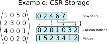
When representing users with no ratings, we repeat the same value in the $indptr$ array, and handle that as a special case in our kernel.

Input Data

Our program accepts CSV files that are formatted as $user\_id,item\_id,ratings$ tuples, wherein both $user\_id$ and $item\_id$ are sequential numerical ids starting from 1, and are sorted based on $user\_id$. For convenience, we provide a script that convert non-sequential ids to sequential ids, and a script that sorts the tuples based on $user\_id$.

The program also needs two different files, one as a training set with which the MF model is trained, and a test set with which the model is evaluated. We use a completely random split across all tuples for generating these files, and split the data into 80% training and 20% test set. We also provide a script to split the data.

Overview

The cu2rec code is organized into 3 main parts: reading in data into sparse matrix form and moving it to the GPU, using SGD and Loss kernels to train the MF model, and moving data back to the host in order to write the trained components to files.

When a user runs cu2rec, they need to supply the train and test CSV files. cu2rec starts by reading both files into a vector of Rating structs that live in the host memory. It then converts each vector of Ratings into a CSR representation. Next, it moves these matrices into the GPU’s memory. Once the memory allocation is complete, cu2rec then loads in the hyperparameters from a config file into constant memory.

Next, cu2rec calls a $train$ function that is responsible for using the sparse rating matrices to train a MF model. $train$ starts by initializing all of the components randomly using a normal distribution with mean of 0 and standard deviation of 1. For the $P$ and $Q$ matrices, these values are normalized by the number of factors the model will use. Next, all of these components are moved to the GPU’s global memory using standard CUDA API functions. Each is wrapped in a helper function to check for CUDA errors. In addition to moving needed memory to the GPU, cu2rec also initializes a CUDA Random object and other needed variables to handle an adaptive learning rate. Finally, the iterative training of the model can begin.

The main training loop in cu2rec does $totalIterations$ loops over two main steps: update components using SGD and computer total losses. cu2rec parallelizes over the number of users in the matrix for both steps. At the beginning of each iteration, the SGD Kernel is called (algorithm 1). The code for the SGD Kernel is below.

1) SGD Kernel

In order for SGD to compute updates to the feature matrices, we needed to create a function that kernels can use to compute a predicted rating using the current components. The code for the Prediction Kernel is below.

2) Prediction Kernel

After running SGD for one item for every user, the algorithm checks if it is time to test the updated model on the test ratings (algorithm 3). This is only done periodically, as computing the total losses is expensive because it needs to compute the error on all ratings, not just one rating per user such as in SGD. To do this, cu2rec first uses the Loss Kernel to compute the loss on every rating.

3) Loss Kernel

Next, cu2rec uses the Total Loss Kernel to reduce all the individual losses so RMSE and MAE can be computed.

4) Total Loss Kernel

After computing the new error metrics, cu2rec checks to see if the learning rate should be lowered by checking a patience counter. Finally, cu2rec swaps the pointers of the updated $Q$ and $itemBias$ components because we want to use the new values for the next round of updating. We do not need to keep copies of $P$ and $userBias$ matrices as the updates are simply done on the original matrices. We only keep a target version of $Q$ and $itemBias$ as updates will have race conditions between threads. More is discussed about this in the next section, Early Bird Gets the Gradient.

Once $totalIterations$ of the training loop are complete, it is time to save the trained model and free all necessary memory. First, all the trained components are copied back to the host variables. Next, the CUDA variables are freed along with all host variables that are not part of the trained model. Outside of the $train$ method, the main code is responsible for writing to file all necessary components of the model that can be used to serve recommendations. The necessary components to write to file are: $P$, $Q$, $userBias$, $itemBias$, and $globalBias$. Once all have been written to a file, cu2rec’s final steps are to free those variables memories on the host and terminate the program.

Early Bird Gets the Gradient

Due to the sequential nature of SGD, we had to come up with a technique to implement SGD with multiple threads potentially trying to update the features of the same item. In SGD, a single error is computed for a rating and both the user corresponding to that rating and the item have their feature matrices and bias weights updated. Because cu2rec parallelizes over users and each user picks a random item they have rated, the same item (especially popular items) is highly likely to be picked by multiple threads. The chance of this becomes near certain with non-trivial amounts of users and is guaranteed if you have more users than items due to the Pigeon Hole principle.

In order to handle race conditions on the same memory, we created the Early Bird Gets the Gradient technique. In the SGD Kernel (algorithm 1), each thread picks a random item from the user’s rated items. Then, it computes the error using the current feature matrices and takes the difference with the true rating. Next, it uses this error to update all of the features. Updating the $P$ matrix and $userBias$ values will never have write conflicts since each thread is responsible for a single user. However, updates to values in $Q$ and $itemBias$ matrices requires special care.

In EBGTG, the first thread to pick an item wins the race to write to that item. To implement this, we created a new boolean array, $itemIsUpdated$, that stores a true or false value for if an item’s features have already been updated. When a thread selects a random item, they check the value in the array and set a local $earlyBird$ variable to $true$ if they ‘won the race.’ They then set the value for this item to $true$ so other threads will set their $earlyBird$ variables to $false$. Threads then only waste time doing $f$ global memory writes to $Q$ and one global memory write to $itemBias[y]$.

However, it should be noted that due to warp divergence, even if a single thread in a warp is selected as the early bird, all threads in the warp are blocked until the early bird thread is finished updating $QTrgt$. Warp divergence is a dangerous occurrence in GPUs when branch conditions are introduced into kernels. In a GPU, threads are bundled into a group of threads, usually 32, that is called a warp. Every thread in a warp executes each instruction of a kernel in lockstep. When a conditional is reached, the GPU has no choice but to block all threads that fail that conditional while all the threads that pass it perform all the instructions in that block of code. Then, when the conditional ends, all the threads begin again performing the remaining instructions in the kernel. Therefore, with EBGTG, if a single thread in a warp is the ‘early bird’, all other threads will be blocked until that single thread does the slow global memory writes.

We were worried at first that warp divergence would prevent any speedup from EBGTG versus Early Bird Loses the Gradient, but in empirical testing, we saw a consistent 12-15% speedup for the entire program.

Advanced Techniques

To optimize run-time and ensure best in class results on test sets, cu2rec utilizes multiple advanced techniques. The use of constant memory, registers, and an optimized reduction sum kernel use the GPU’s architecture to greater advantage. Our parallel lock-free updates and user index striding ensure we achieve the best results possible against test set ratings.

Constant Memory

All of our kernels rely on many of the same static variables, such as hyper parameters and dimensions. These values include total iterations, number of factors, $\eta$, $\lambda_p$, $\lambda_q$, $\lambda_u$, and $\lambda_i$.

The constant memory is useful because from the kernel’s point of view, it never changes, and can therefore be aggressively cached. Because all of the values we store in constant memory never change during the execution of cu2rec, all of these values get cached in the beginning of execution and remain in the cache for the runtime of the program.

Aggressive Register Use

Registers are the fastest memory available on the GPU and accesses to this memory can be over 100x faster than global memory¹. As such, one of our goals was to aggressively use registers to store any values that are used more than once in a kernel. We will break down which values we decided to store in registers.

In the SGD Kernel (algorithm 1), the following variables are created to store values in registers: $x$ (the user id), $low$ (the first rated item id index pointer), $high$ (the last rated item id index pointer), $yi$ (random item index pointer), $y$ (the item id), $ub$ (user $x$’s bias), $ib$ (item $y$’s bias), $error$ (the error of the model on the rating of user x on item y), $earlyBird$ (if the user is first to update item’s features), $pOld$ (old value for feature matrix $P$ at row $x$ and column $i$), and $qOld$ (old value for feature matrix $Q$ at row $y$ and column $i$).

In the Loss Kernel (algorithm 3), the following variables are created to store values in registers: $x$ (the user id), $ub$ (user $x$’s bias), and $itemId$ (the item index for every item $x$ has rated).

We experimented with having less register use, thinking it might allow for more blocks to be scheduled at the same time, but that resulted in more global memory accesses (and more pressure on the caches), and was overall empirically slower.

Reduction Sum

The total loss kernel, which is used to calculate the global loss after a set number of updates, uses a fixed number of threads $t_g$ per grid regardless of the number of ratings. This makes it easy to scale to very high number of ratings ($N$). It uses the reduction sum technique, wherein each thread at each step calculates a partial sum of its previous partial sum and the next thread’s previous partial sum. This is done for $log(N)$ steps.

Each thread initially calculates the sum of $N/t$ elements sequentially, where each element is $t_g$ apart from the previous one, allowing coalesced memory accesses. These sums are written into the shared memory.

After this step, each block (size $t_b$) reduces its own sum into the sum at $tid=0$. This is done for $log(N)$ steps, wherein in the first step, the first $t_b/2$ threads calculate their partial some with the sums in $tid$ and $tid + t_b/2$, and then $t_b/4$ threads, and so on. This approach coalesces the memory accesses and minimizes branch divergence. We also use loop unrolling to reduce the number of if statements, and also use templating with the block size to get rid of the unnecessary unrolled checks in compile-time.

At the end, each thread with $tid=0$ writes its own sum to the global memory, so we get a partial sum per block. These can be fed into another reduce sum kernel, but we found doing the final addition on the host was faster.

Parallel Lock-Free Updates

As discussed in the section explaining Early Bird Gets the Gradient, cu2rec does not lock any memory address writes while updating feature matrix weights. Earlier versions of cu2rec utilized atomic operations to update the $Q$ and $itemBias$ matrices. However, after discovering that optimal results could be achieved by simply letting a single thread ‘win’ an update, we decided to remove any atomic operations from any kernel.

User Index Striding

EBGTG favors whichever thread selects an item first and sets the $itemIdUpdated$ value to $true$. Therefore, we must ensure that every thread (and therefore every user) gets a fair shot to be the ‘early bird.’ At first, with naive EBGTG, we were seeing 2-3% worse results on test data than other implementations. This gap in results increased for larger datasets, including almost 8% worse results on the Netflix Dataset when compared to best in class results⁹. We learned that EBGTG was scheduling lower index users first since they would always be in the first few blocks every iteration. While there is no guarantee which blocks begin running first, there are limited SMs on a GPU and therefore some blocks are queued while waiting to run. We found that later users would consistently be scheduled to higher block indexes, and thus run last.

In order to combat this, we decided to offset which user each thread uses to perform SGD. In the training loop, we add an offset variable every iteration and pass that to the SGD kernel (algorithm 1). This effect can be seen in the first line where $x$ is computed. What this offset does is ensure that over time, every thread will be responsible for different sections of the user matrix.

By implementing this striding, we immediately began to see equal results in test set error metrics compared to other well known implementations.

Results

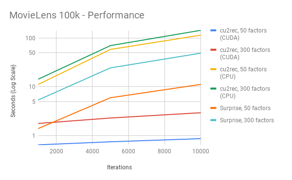
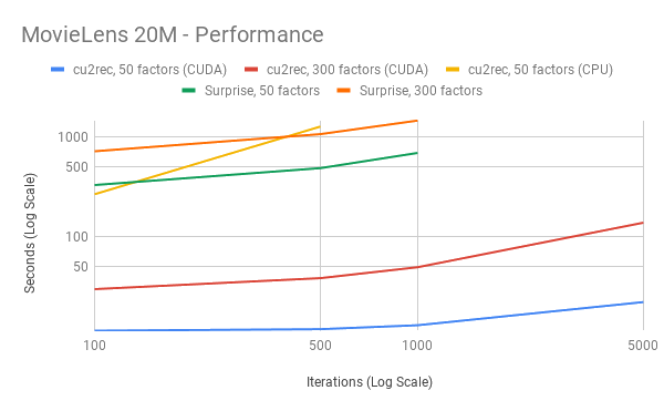
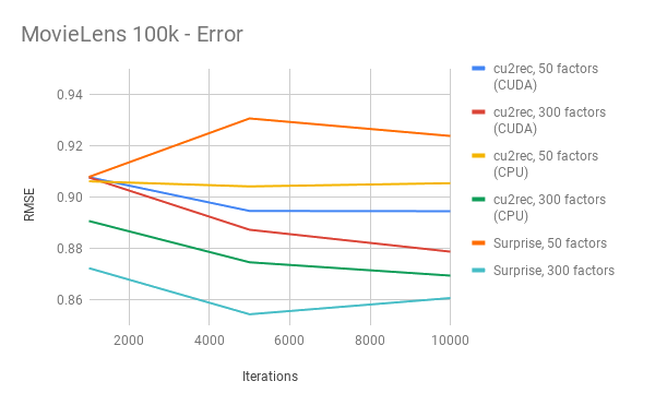
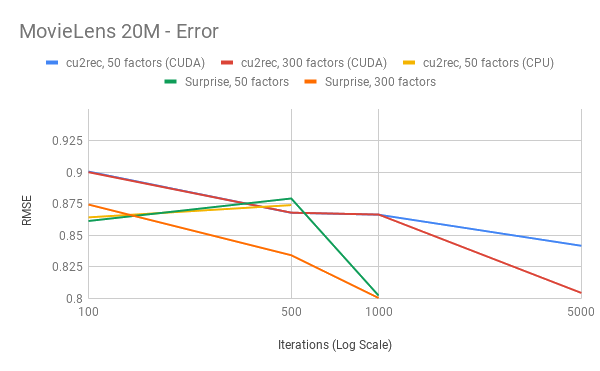
We benchmarked our GPU code using an NVIDIA V100 GPU, and the CPU code with an Intel i7-6650U CPU.

Speedup

Comparison of total time on ML-100k

Comparison of total time on ML-20M

RMSE

Comparison of RMSE on ML-100k

Comparison of RMSE on ML-20M

GPU vs GPU

We tested our code both with a V100 on NYU’s Prince server, and a TITAN Z in NYU’s cuda2 server. We varied problem sizes, the memory bandwidth requirements, and the number of iterations to get a healthy comparison. This is visualized in the following figure:

Comparison of speedup on different problem sizes

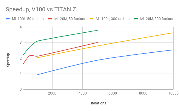
The V100 has 5,120 CUDA cores vs 5,760 of TITAN Z, 900GB/s memory bandwidth vs 672GB/s of TITAN Z, and higher clock speed.

In terms of the cost in performance, going from the ML-100k to ML-20M dataset increases the total problem size, as there are more users, items, and ratings to train for. Holding all other things equal, we would expect a scalable code to have higher speedup with larger problem size, and our speedup satisfies this.

In terms of bandwidth requirement, increasing the number of factors from 50 to 300 has a direct effect on it, because the SGD kernel needs to retrieve more data from the global memory. Holding all other things equal, we would expect a scalable code to have higher speedup with increased memory bandwidth, and our speedup satisfies this.

Conclusion

GPU technology opens the door to massive acceleration for a wide variety of problems. Machine Learning has recently seen a massive boost in effectiveness from both powerful GPUs and the availability of big data to train complex models on. Recommender Systems are an interesting subset of machine learning as they benefit greatly from larger and larger datasets that allow models to uncover complex latent relationships between users and items. SGD is one of the most popular algorithms to optimize recommender system MF models. However, SGD provides a challenging problem for GPU implementations due to its inherent sequential definition.

This blog post introduced cu2rec, a novel parallel implementation of SGD used to solve recommender system matrix factorization. Through the use of a parallel lock free SGD kernel and a variety of advanced CUDA programming techniques, cu2rec achieves a 10x speedup over one of the fastest sequential recommender system MF libraries while matching best in class error metrics. In addition to outperforming sequential implementations of SGD MF, cu2rec has also been shown to scale with better GPU hardware.

References

1. D. B. Kirk and W. H. Wen-Mei, Programming massively parallel processors: a hands-on approach. Morgan kaufmann, 2016. ↩ ↩² ↩³

2. A. Coates, B. Huval, T. Wang, D. Wu, B. Catanzaro, and N. Andrew, “Deep learning with cots hpc systems,” in International Conference on Machine Learning, 2013, pp. 1337–1345. ↩

3. A. Bari, M. Chaouchi, and T. Jung, Predictive analytics for dummies. John Wiley & Sons, 2016. ↩

4. Y. Koren, “The bellkor solution to the netflix grand prize,” Netflix prize documentation, vol. 81, pp. 1–10, 2009 ↩

5. Y. Koren, R. Bell, and C. Volinsky, “Matrix factorization techniques for recommender systems,” Computer, no. 8, pp. 30–37, 2009. ↩

6. W. Tan, L. Cao, and L. L. Fong, “Faster and cheaper: Parallelizing large-scale matrix factorization on gpus,” CoRR, vol. abs/1603.03820, 2016. [Online]. Available: http://arxiv.org/abs/1603.03820 ↩

7. B. Recht, C. Re, S. Wright, and F. Niu, “Hogwild: A lock-free approach to parallelizing stochastic gradient descent,” in Advances in neural information processing systems, 2011, pp. 693–701. ↩ ↩²

8. H. Yun, H. Yu, C. Hsieh, S. V. N. Vishwanathan, and I. S. Dhillon, “NOMAD: non-locking, stochastic multi-machine algorithm for asynchronous and decentralized matrix completion,” CoRR, vol. abs/1312.0193, 2013. [Online]. Available: http://arxiv.org/abs/1312.0193 ↩

9. X. Xie, W. Tan, L. L. Fong, and Y. Liang, “Cumf sgd: Fast and scalable matrix factorization,” CoRR, vol. abs/1610.05838, 2016. [Online]. Available: http://arxiv.org/abs/1610.05838 ↩